This function builds a map that visualises the probability of exceeding some nominated threshold of concern.
build_emap(
  data,
  pdflist = NULL,
  geoData = NULL,
  id = NULL,
  key_label,
  palette = "YlOrRd",
  size = NULL,
  border = NULL
)
Arguments
- data
A data frame containing columns that house estimates of the mean, standard deviation (or margin of error) and exceedance probability (optional). A number of options are considered for calculating the probability of exceeding a threshold. See below for more information.
- pdflist
A list capturing the pdf function that defines the distribution function to use to calculate the probabilities of exceedance. By default this is NULL and assumes the exceedance probabilities have been calculated outside of the function and passed as a third column of the data frame. Functions need to conform to the class of distribution functions available within R through the
statspackage.- geoData
An sf or sp object.
- id
Name of the common column shared by the objects passed to
dataandgeoData. The exceedance probability in the data frame will be matched to the geographical regions through this column.- key_label
Label of legend.
- palette
Name of colour palette. Colour palette names include
"YlOrBr","YlOrRd","YlGnBu"and"PuBuGn".- size
An integer between 1 and 20. Value controls the size of points when
geoData = NULL. Ifsize = NULL, the points will remain the default size.@details An exceedance probability map can be produced using: (i) precalculated exceedance probabilities, which are provided as a third column to the input dataframe; or (ii) exceedance probabilities that are calculated within the function using one of the standard probability distributions (e.g.
pnorm) provided in thestatspackage in R, or (iii) exceedance probabilities that are calculated through a user defined function that is passed to the package which conforms to a similar structure as the suite ofDistributionsavailable in R. Examples are provided below.- border
Name of geographical borders to be added to the map. It must be one of
county,france,italy,nz,state,usaorworld(see documentation formap_datafor more information). The borders will be refined to match latitute and longtidue coordinates from the geoData argument.
Details
If geoData remains NULL, the function will produce a map of
plotted points representing specific sites; in this case, the data frame must
include latitude and longitude coordinates in columns "long" and
"lat".
Examples
data(us_data)
data(us_geo)
poverty <- read.uv(data = us_data, estimate = "pov_rate", error = "pov_moe")
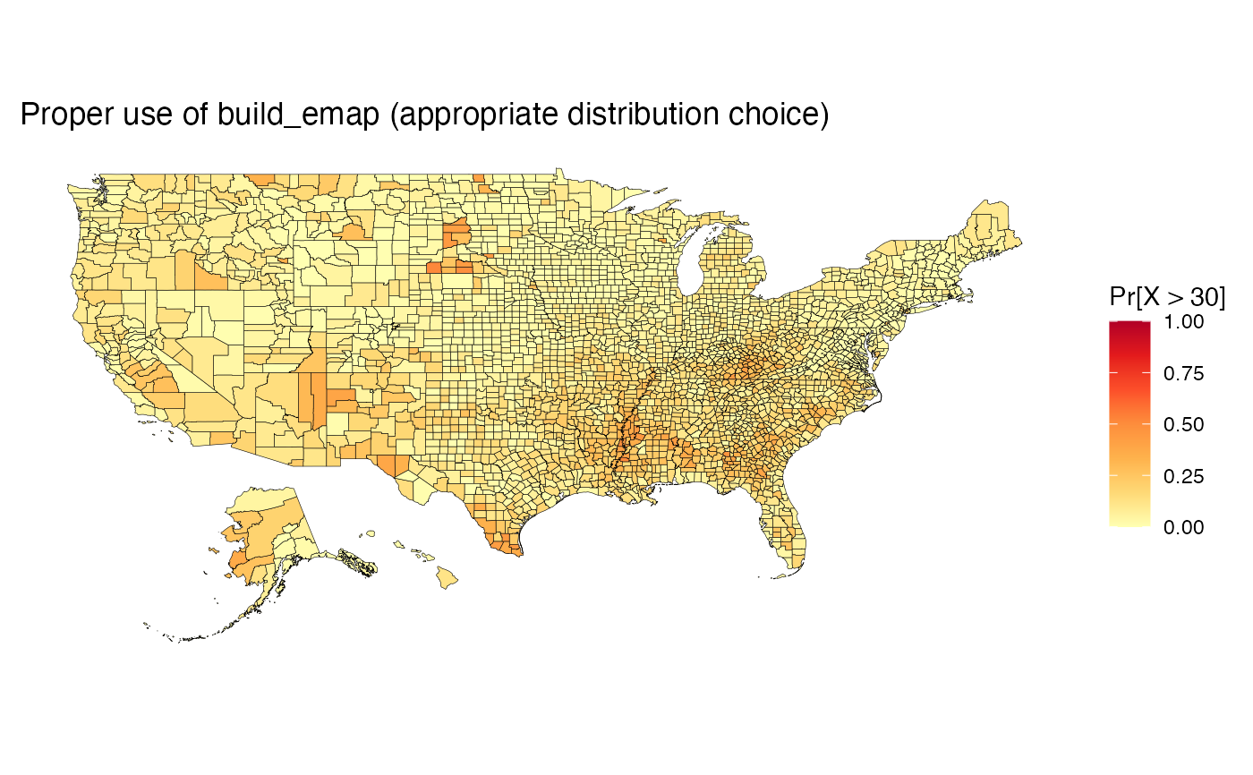
# Exceedance probability map: Pr[X > 30] (Exponential Distribution)
#---- define probability distribution
pd <- quote({ pexp(q, rate, lower.tail = FALSE) })
#---- define argument listing
args <- quote({ list(rate = 1/estimate) })
#---- capture distribution and arguments in a single list
pdflist <- list(dist = pd, args = args, th = 30)
map <- build_emap(data = poverty, pdflist = pdflist, geoData = us_geo, id = "GEO_ID",
border = "state", key_label = "Pr[X > 30]")
#> Warning: Ensure the pdf you select is suitable for your data. See ??build_emap for examples of good and bad distribution choices.
view(map) + ggplot2::ggtitle("Proper use of build_emap (appropriate distribution choice)")
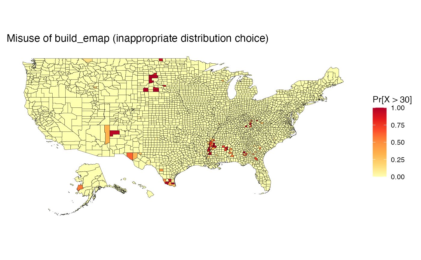
 # Example where an inappropriate distributions is tried
# Exceedance probability map: Pr[X>30] (Normal Distribution)
#---- define probability distribution
pd <- quote({ pnorm(q, mean, sd, lower.tail = FALSE) })
#---- define argument listing
args <- quote({ list(mean = estimate, sd = error/1.645) })
#---- capture distribution and arguments in a single list
pdflist <- list(dist = pd, args = args, th = 30)
map <- build_emap(data = poverty, pdflist = pdflist, geoData = us_geo, id = "GEO_ID",
border = "state", key_label = "Pr[X > 30]")
#> Warning: Ensure the pdf you select is suitable for your data. See ??build_emap for examples of good and bad distribution choices.
view(map) + ggplot2::ggtitle("Misuse of build_emap (inappropriate distribution choice)")
# Example where an inappropriate distributions is tried
# Exceedance probability map: Pr[X>30] (Normal Distribution)
#---- define probability distribution
pd <- quote({ pnorm(q, mean, sd, lower.tail = FALSE) })
#---- define argument listing
args <- quote({ list(mean = estimate, sd = error/1.645) })
#---- capture distribution and arguments in a single list
pdflist <- list(dist = pd, args = args, th = 30)
map <- build_emap(data = poverty, pdflist = pdflist, geoData = us_geo, id = "GEO_ID",
border = "state", key_label = "Pr[X > 30]")
#> Warning: Ensure the pdf you select is suitable for your data. See ??build_emap for examples of good and bad distribution choices.
view(map) + ggplot2::ggtitle("Misuse of build_emap (inappropriate distribution choice)")
 # Example where exceedance probabilities have been supplied (GBR Example)
# Load Upper Burdekin Data
data(UB)
# Build Palette
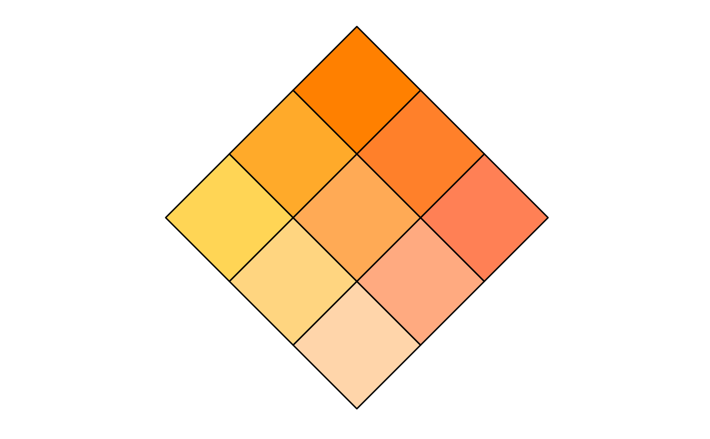
exc_pal <- build_palette(name = "usr", colrange = list(colour = c("yellow", "red"),
difC = c(1, 1)))
view(exc_pal)
# Example where exceedance probabilities have been supplied (GBR Example)
# Load Upper Burdekin Data
data(UB)
# Build Palette
exc_pal <- build_palette(name = "usr", colrange = list(colour = c("yellow", "red"),
difC = c(1, 1)))
view(exc_pal)
 # Create map and view it
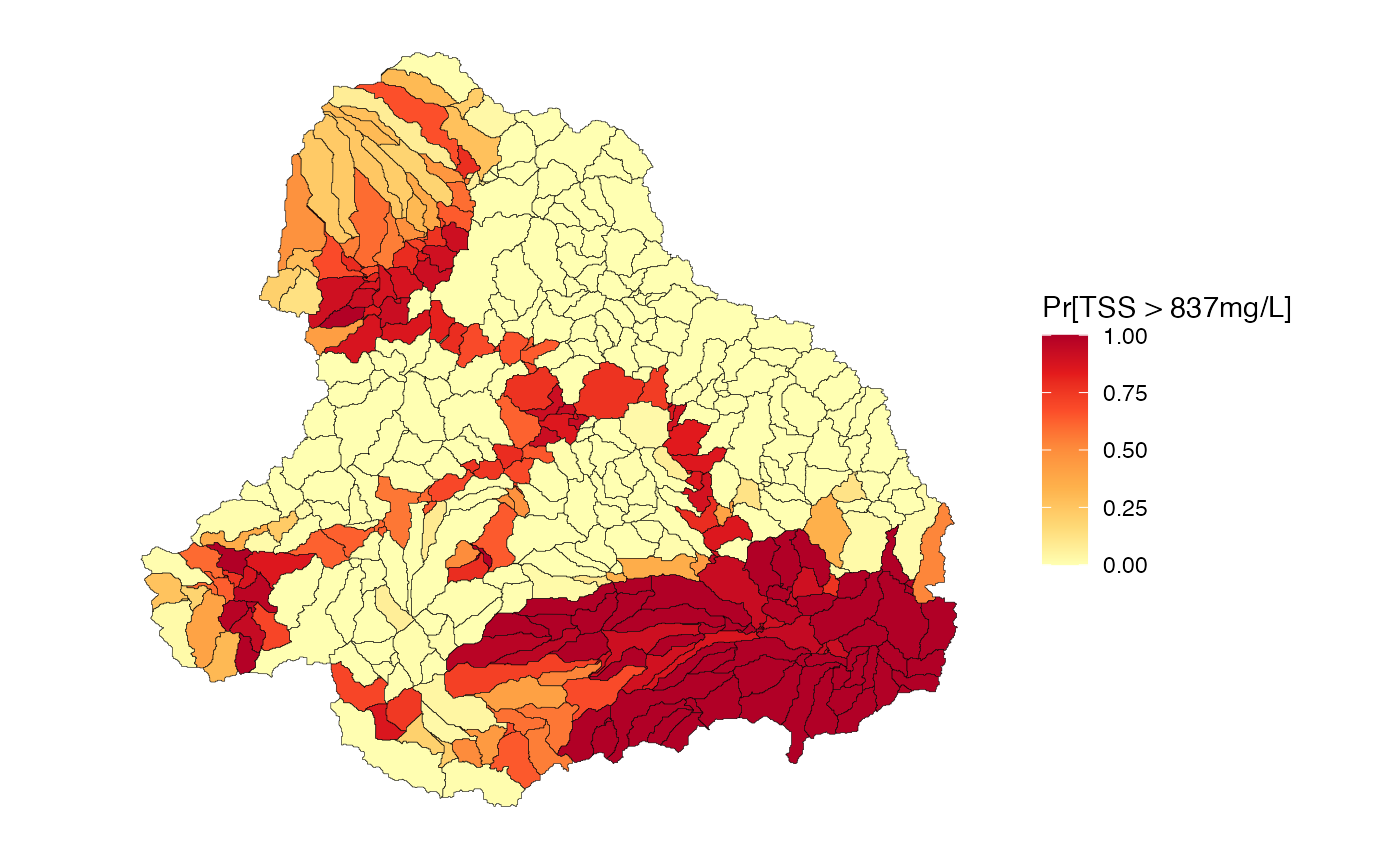
tss <- read.uv(data = UB_tss, estimate = "TSS", error = "TSS Error", exceedance = "TSS_exc1")
map <- build_emap(data = tss, geoData = UB_shp, id = "scID",
key_label = "Pr[TSS > 837mg/L]")
view(map)
# Create map and view it
tss <- read.uv(data = UB_tss, estimate = "TSS", error = "TSS Error", exceedance = "TSS_exc1")
map <- build_emap(data = tss, geoData = UB_shp, id = "scID",
key_label = "Pr[TSS > 837mg/L]")
view(map)