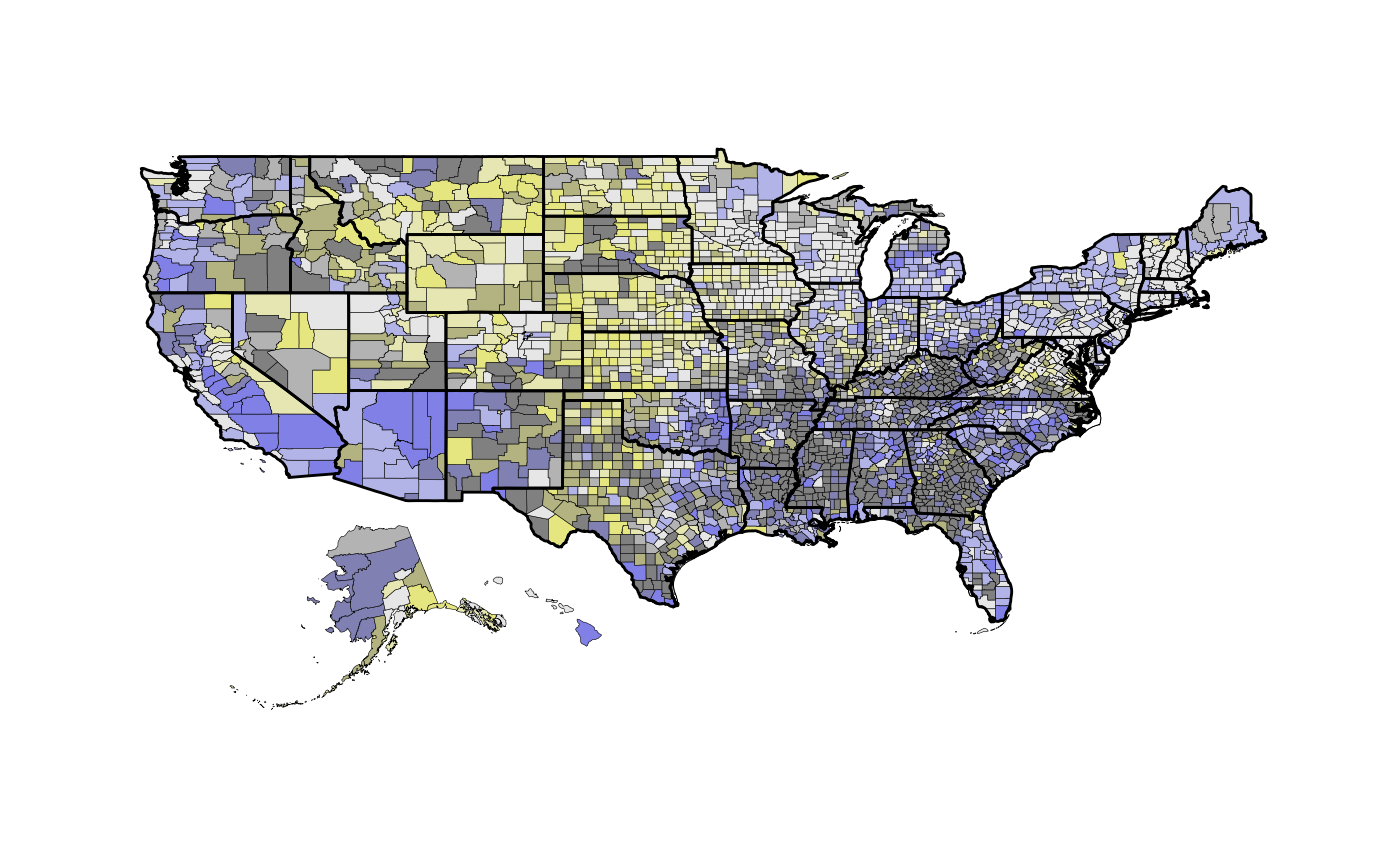
This function builds a map that visualises estimates and errors simultaneously with a bivariate colour scheme.
build_bmap(
  data,
  geoData = NULL,
  id = NULL,
  border = NULL,
  palette = "BlueYellow",
  size = NULL,
  terciles = FALSE,
  bound = NULL,
  flipAxis = FALSE
)
Arguments
- data
A data frame with estimates and errors, formatted with
read.uv.- geoData
An sf or sp object.
- id
Name of the common column shared by the objects passed to
dataandgeoData. The estimates and errors in the data frame will be matched to the geographical regions through this column.- border
Name of geographical borders to be added to the map. It must be one of
county,france,italy,nz,state,usaorworld(see documentation formap_datafor more information). The borders will be refined to match latitute and longtidue coordinates from the geoData argument.- palette
Name of colour palette or character vector of hex colour codes from the
build_palettefunction. Colour palette names includeBlueYellow,CyanMagenta,BlueRedandGreenBlue.- size
An integer between 1 and 20. Value controls the size of points when
geoData = NULL. Ifsize = NULL, the points will remain the default size.- terciles
A logical value. This provides the option to define numerical bounds for the colour key grid using terciles instead of equal intervals.
- bound
Output from the
findNboundsfunction if a different set of data is required to bound the map. This is useful if you are wanting to create a bivariate map across multiple years and show colours that correspond to the same key. Default is NULL.- flipAxis
A logical value. Whether to place the axis on the opposite sides or not.
Details
If geoData remains NULL, the function will produce a map of
plotted points representing specific sites; in this case, the data frame must
include latitude and longitude coordinates in columns "long" and
"lat".
